Simulations with Wave Loads

One of the main features of the mclsimpy library is to simulate vessels with wave loads. Using the mclsimpy.waves packages, we can generate sea states by from wave spectras, and calculate the loads on the vessel. Here, laods refer to the first- and second-order wave loads.

We will in this tutorial show how to create a sea state, and how to use it to simulate a vessel subject to wave loads.

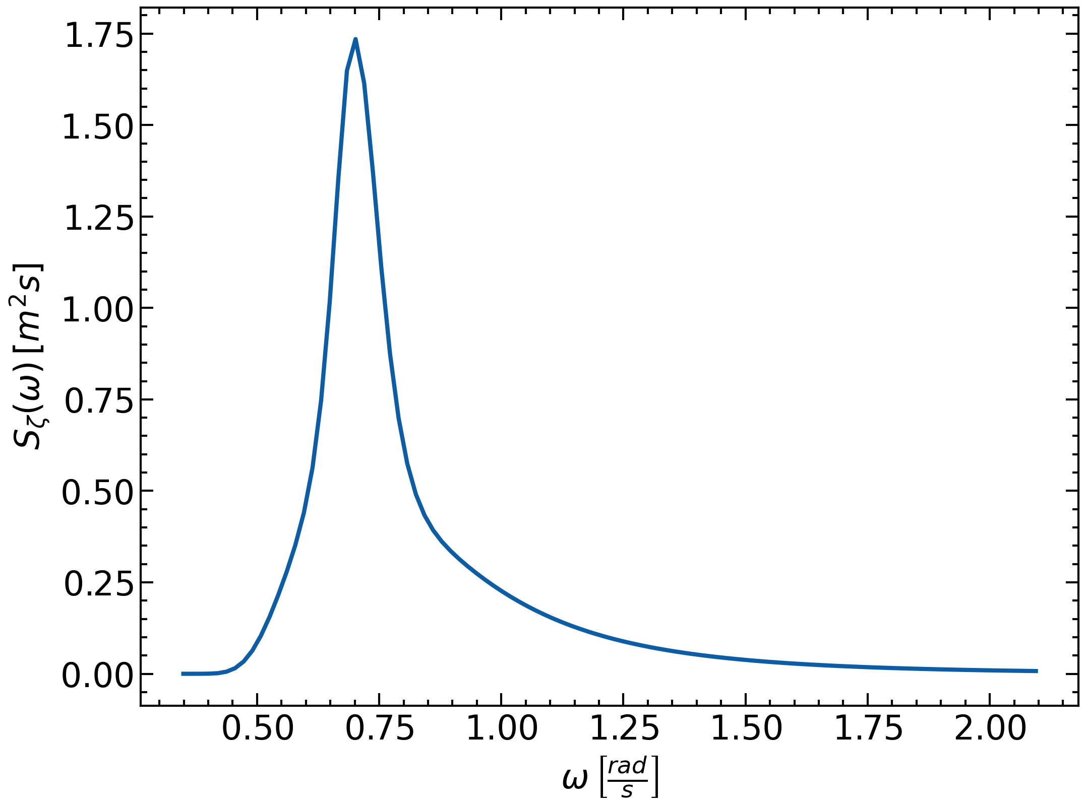
First, we will generate a sea state with 100 wave components. We will in this example use the JONSWAP wave spectra. The number of wave components should be selected based on the simulation time and the time step used. A larger number of wave components must be used for longer simulations.

from mclsimpy.waves import JONSWAP
import numpy as np

hs = 2.5    # Signifcant wave height
tp = 9.0    # Peak wave period
gamma = 3.3 # Peakedness factor of wave spectra
wp = 2*np.pi/tp

wmin = 0.5*wp
wmax = 3.0*wp

N = 100     # Number of wave components

wave_freqs = np.linspace(wmin, wmax, N)

jonswap = JONSWAP(wave_freqs)

_, wave_spectrum = jonswap(hs=hs, tp=tp, gamma=gamma)

Having defined the wave spectrum, we can compute the wave amplitudes using the simple relation:

\[\zeta_{a,i} = \sqrt{2S(\omega_i)d\omega}.\]

We will define a set of random phases (representing the random phase difference between each wave) and define a set of wave angles. In this example, we will model long-crested sea (unidirectional waves). The wave direction is defined in the NED frame as waves-going-to. A wave anlge of 0 rad represents a wave moving in the North direction, while an angle PI represents waves moving in South direction. Note that the angle is defined positive in the clockwise direction from North.

Before we create the WaveLoad object, we will instantiate a Vessel object. This is due to the fact that the WaveLoad object requires a configuration file with vessel specific RAOs. In this example, we are using the RV Gunnerus 6 DOF simulation model.

from mclsimpy.simulator import RVG_DP_6DOF
from mclsimpy.waves import WaveLoad

# Set the simulation parameters
dt = 0.1    # Simulation time step to be used
simtime = 600   # 10 minute simulation
time = np.arange(0, simtime, dt)

vessel = RVG_DP_6DOF(dt, method="RK4") # RVG model with RK4 intergration method.

dw = (wmax - wmin)/N      # Space between each frequency component
wave_amps = np.sqrt(2*wave_spectra*dw)   # Calculate wave amplitudes
rand_phase = np.random.uniform(0, 2*np.pi, size=N)
wave_angles = np.ones(N)*np.pi # Waves going south

waveload = WaveLoad(
    amps=wave_amps,
    freqs=wave_freqs,
    eps=rand_phase,
    angles=wave_angles,
    config_file=vessel._config_file,
    interpolate=True,
    qtf_method="geo-mean",      # Use geometric mean to approximate the QTF matrices.
    deep_water=True
)

Having created a Vessel and related WaveLoads object, we can start the simulation. This can be done using a simple for loop.

eta = np.zeros((len(time), 6))  # Array to store the vessel positions

# Define 0 current for this simulation
Uc = 0.0
betac = 0.0

for i in range(1, len(time)):
    # Compute the first and second order wave loads
    tau_wave = waveload(time[i], vessel.get_eta())

    # Alternatively, compute first and second-order loads separately
    # tau_wf = waveload.first_order_loads(time[i], vessel.get_eta())
    # tau_sv = waveload.second_order_loads(time[i], vessel.get_eta()[-1])

    vessel.integrate(Uc, betac, tau_wave)

    eta[i] = vessel.get_eta()

And that’s it. As simple as it gets :D. The simulation can of course be expanded to include other loads such as thurster loads.